`IPEDtaS` Tutorial

This page will walk you the basics of how to use IPEDtaS to automagically retrieve labelled IPEDS .dta files

What `IPEDtaS` Does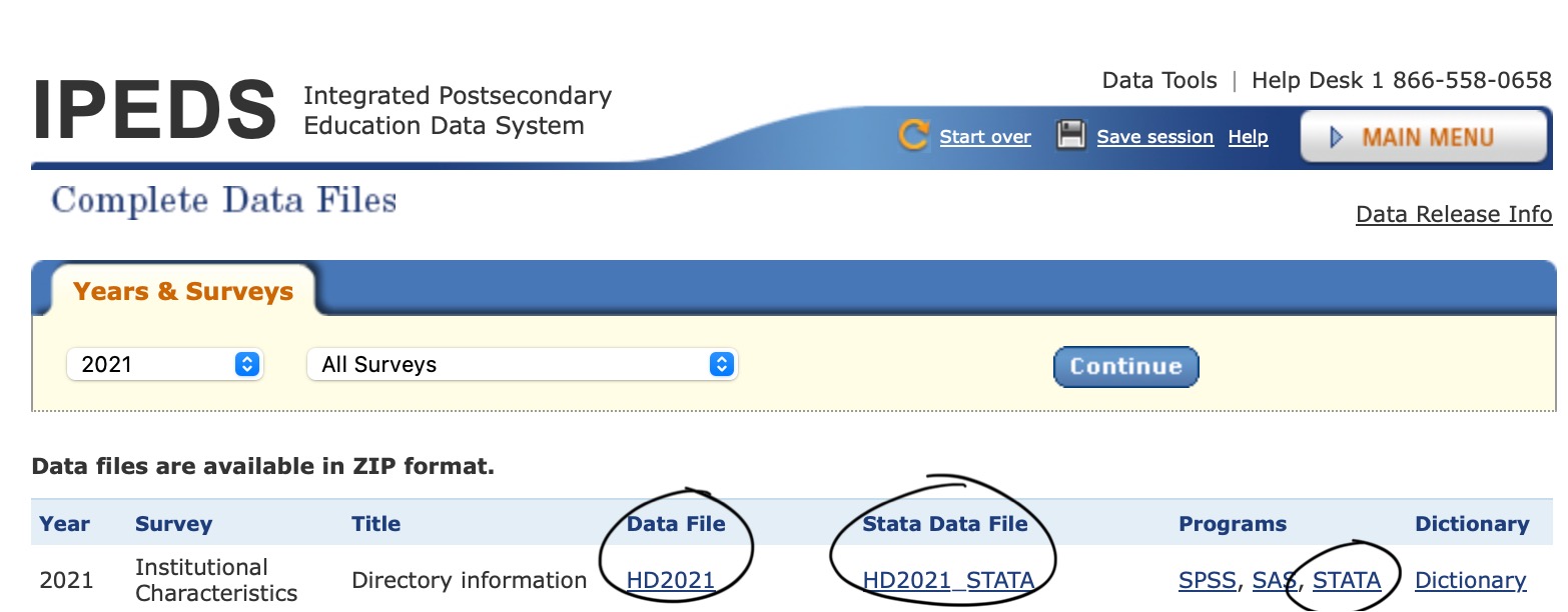

NCES provide all the information needed to create labelled IPEDS data
- However, it can be cumbersome to put all the pieces together manually
If you’ve worked with IPEDS before, you’ve likely seen this screen
When I first started working with IPEDS, I assume the “Stata Data File” would be a nicely labelled data set, like you can get with other NCES data sets
- However, it’s not
- Instead, it’s just a plain .csv data set that is designed to be combined with the “STATA Program File” which applies the labels
  - These program files are also full of issues
    - Such as hard coded file paths from the NCES worker who wrote the script’s computer which you would have to update for each piece of data
    - And error-causing line breaks which you’d have to fix before the script would run
- Between downloading two files, fixing the issues, then running them together, it’s a lot of work so most people don’t bother
- Plus, they only work in Stata, R users without a Stata license are left out…
The R and Stata IPEDtaS scripts do all this heavy lifting for you so you can use nicely labelled IPEDS data without the extra effort!

Why Would I Want Labels Any?

You will see more of this in the applied example below, but, in short, they make data analysis much easier and reduce the amount you will have to look at the dictionary/codebook!

Look at the difference from these simple data checks on the number of colleges in each region

Without labels, we just get the numeric code for each region which we’d have to look up

data_without_labels |>
  count(obereg)

# A tibble: 10 × 2
   obereg     n
    <dbl> <int>
 1      0     7
 2      1   337
 3      2  1025
 4      3   891
 5      4   491
 6      5  1536
 7      6   665
 8      7   236
 9      8   953
10      9   148

With labels, we get a description of each region too

data_with_labels |>
  count(obereg)

# A tibble: 10 × 2
   obereg                                                             n
   <dbl+lbl>                                                      <int>
 1 0 [U.S. Service schools]                                           7
 2 1 [New England (CT, ME, MA, NH, RI, VT)]                         337
 3 2 [Mid East (DE, DC, MD, NJ, NY, PA)]                           1025
 4 3 [Great Lakes (IL, IN, MI, OH, WI)]                             891
 5 4 [Plains (IA, KS, MN, MO, NE, ND, SD)]                          491
 6 5 [Southeast (AL, AR, FL, GA, KY, LA, MS, NC, SC, TN, VA, WV)]  1536
 7 6 [Southwest (AZ, NM, OK, TX)]                                   665
 8 7 [Rocky Mountains (CO, ID, MT, UT, WY)]                         236
 9 8 [Far West (AK, CA, HI, NV, OR, WA)]                            953
10 9 [Other U.S. jurisdictions (AS, FM, GU, MH, MP, PR, PW, VI)]    148

First, this makes life easier reducing the amount we have to look back and forth to the code book
Second, it makes it easier to spot accidental errors when checking our work, leading to more reliable analyses

System Requirements

First things first, let’s consider the what you will need on your computer to get started

R
Stata

An up-to-date version of R
- If you’re not sure how up-to-date your R is, download a new version of R from https://cran.r-project.org
An up-to-date tidyverse package
- In your R console type install.packages("tidyverse") to get the latest version
If you want to download all of IPEDS, up to 12gb of permanent space and 36gb of temporary space

An up-to-date and licensed copy of Stata version 16.0 or higher (BE or Basic is sufficient)
- You can upgrade/purchase/download Stata from https://www.stata.com
An up-to-date installation of Python
- Don’t fret, you don’t have to use Python, but the .do file uses PyStata to clean up the scripts, so Python just needs to be on your machine
- You can see if you already have Python by typing python search into your Stata command box
- You can install a copy of Python from https://www.python.org/downloads/
If you want to download all of IPEDS, up to 4gb of permanent space and 12gb of temporary space

Setting up Your Project Folder

This part is identical for both Stata and R users, the main points to note are:

Download either the Stata or R version of the script from the links at the top of this page

Hint: If the file is opening in your browser, use “download linked file” on macOS, or, “save link as” on windows to save the file (you can also just copy and paste)

The script is designed to treat where ever you place the IPEDtaS.do or IPEDtaS.R file as the “working directory”

Check the working directory is set to your current project before doing anything else
- If you download the script, save it in your project folder, then open it, you will often get the correct working directory by default, but it’s always best to check
- When the script runs it will store output in ./data and ./dictionaries folders
  - Caution: Anything you have in folders with that name will be overwritten
  - This also applies to ./zip-data, ./zip-do-files, ./zip-dictionaries, ./unzip-data, ./unzip-do-files, ./unzip-dictionaries which are folders used temporarily behind-the-scenes

Personally, I set up my projects with scripts in the top-level of the project folder (as in, not in a sub-folder), so that is how IPEDtaS was designed
- If you need everything in a sub-folder for sanity reasons either:
  1. Place IPEDtaS in your data folder (e.g ./data/IPEDtaS.do) which will place the data in ./data/data/hd2022.dta
  2. Place IPEDtaS in your ./scripts folder and go through adjusting all the relative paths by adding ../ to back out one level

File Selection

The only real change you have to make in the whole process is to the scripts is selecting which files you want to download

By default the scripts are set to download directory information (HD) and enrollment data (EFFY) for the 2023 reporting cycle
- To change these you need to update the list to the files you want
- Note: at the bottom of the script there is a list with every single IPEDS file in it, if you want the entire dataset you can just copy and paste that longer list to the top of the script and edit as needed
To edit the list you basically just need to follow the list rules for each language

R
Stata

The only rule is that the selected_files <- c() must be a valid list of IPEDS file names
- Each line/entry must end in a comma , except the final one

Here are some short examples of file selection

A simple list

selected_files <- c("HD2021", "EFFY2022", "SFA2122")

## OR

selected_files <- c(
  "HD2021",
  "EFFY2022",
  "SFA2122"
)

You can also comment out files you don’t want from a longer list

selected_files <- c(
  "HD2021",
  # "IC2022",
  # "IC2022_AY",
  "EFFY2022",
  # "EFFY2022_DIST",
  "SFA2122"
)

That’s about it, when you run the script, the files you put in selected_files will be downloaded

For the Stata version local selected_files needs to be a valid list of IPEDS file names
- Each line in the list must end in /// except the final one

Here are some short examples of file selection

A simple list

local selected_files ///
  "HD2021" ///
  "EFFY2022" ///
  "SFA2122"

Use multi-line comments to comment out files you don’t want

Stata has both single-line comments // or * and multi-line commments which start /* and end */
- Because of the way the list is structured, we have to use multi-line comments here (even to comment a single line) which have 3 rules
1. To work in the list, the line before a multi-line comment must be /// and nothing else
2. Below this start the first line of a multi-line comment with /*
3. To close out a multi-line comment somewhere else use */

local selected_files ///
  "HD2021" ///
  ///
  /*
  "IC2022" ///
  "IC2022_AY" ///
  */
  "EFFY2022" ///
  ///
  /*
  "EFFY2022_DIST" ///
  */
  "SFA2122"

That’s about it, when you run the script, the files you put in local selected_files will be downloaded

Runnning the Script

Once you have the file selection set, simply save the script and hit run/do!

If you’re using this tool as part of a reproducible research project, you might want to include running it as part of your analysis code

However, you don’t want to run it every time you run your code, only if the data isn’t already downloaded
The below code blocks will do exactly that if you include them at the start of your analysis code
- Just change hd2021.dta to a file you download

R
Stata

if(!file.exists("data/hd2021.dta")) { source("IPEDtaS.R") }

if(!fileexists("data/hd2021.dta")) { do "IPEDtaS.do" }

Applied Example Using with Labelled IPEDS Data

Okay, now we have our labelled IPEDS data, let’s walk through a simple descriptive analysis using

HD2021 (institutional characteristics as of Fall 2021)
EFFY2022 (enrollment for 2021-2022 school year)
SFA2022 (financial aid for 2021-2022 school year)

Two things to note:

These examples are just meant to illustrate how the labels can help in your work, they are not meant to be ground-breaking informative analyses - If you’re feeling adventurous, play around and swap out different variables as you follow along
To be able to understand some of the code, you’d a decent understanding of R and the tidyverse, but again, the point is just to see how the labels can help

1. Running `IPEDtaS`, Reading Data, & Joining Data

R
Stata

1. Create a new folder on your computer, download a copy of IPEDtaS.R, and place it in the folder

2. Adjust selected_files <- c() in IPEDtaS.R to download the 3 files we want like below

selected_files <- c(
  "HD2021",
  "EFFY2022",
  "SFA2122"
)

3. Select the whole IPEDtaS.R script and hit “Run”

4. Start a new R script in that same folder

5. Load tidyverse, haven (part of tidyverse, but requires loading separately), labelled (what haven uses behind the scenes), and gtsummary (to easily create output tables)

library(tidyverse)
library(haven)
library(labelled)
library(gtsummary)

6. Read our data in

data_info <- read_dta("data/hd2021.dta")
data_enroll <- read_dta("data/effy2022.dta")
data_aid <- read_dta("data/sfa2122.dta")

Okay, now, take a look at the enrollment data we just read in (click on data_enroll in the environment in the top right)

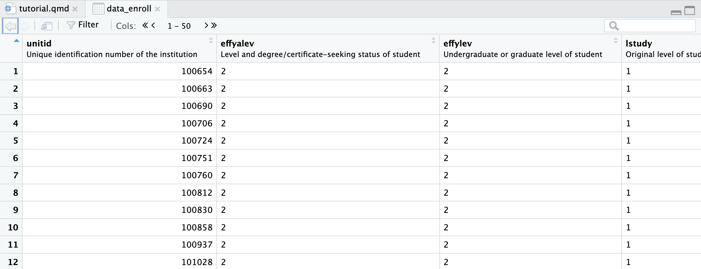
Screenshot of Enrollment Data Showing Variable Labels

Notice the descriptions under each variable name

If you’re familiar with IPEDS data, you won’t be used to seeing those
They’re the variable labels we added, super useful for quick questions without having to open the code book!

7. Now we want to join our data together

data <- left_join(data_info, data_enroll, by = "unitid") |>
  left_join(data_aid, by = "unitid")

1. Create a new folder on your computer, download a copy of IPEDtaS.do, and place it in the folder

2. Adjust local selected_files in IPEDtaS.do to download the 3 files we want like below

local selected_files ///
  "HD2021" ///
  "EFFY2022" ///
  "SFA2122"

3. Select the whole IPEDtaS.do script and hit “Run”

4. Start a new Stata do file in that same folder

5. Load our first data set, hd2022

use "data/hd2021.dta", clear

Okay, now, take a look at the variables panel (by default in right hand panel)

Each of the variables has a label that describes what the variable means
If you’re familiar with standard IPEDS data, you won’t be used to seeing those
They’re the variable labels we added, super useful for quick questions without having to open the code book!

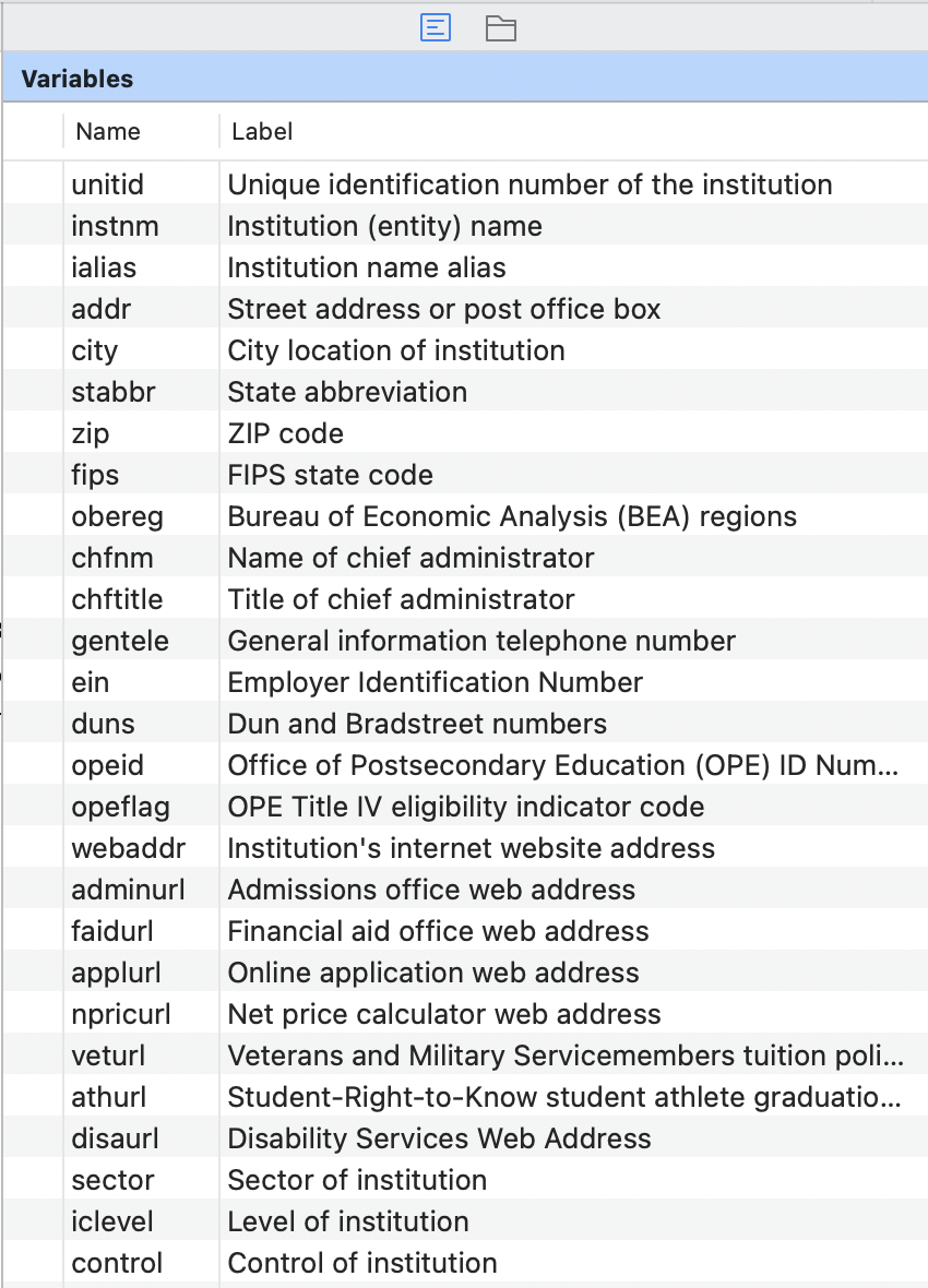
6. Join in our other data sets in a “left join” style (i.e., all observations in the first data set are kept even if they don’t have a match in the second)

joinby unitid using "data/sfa2122.dta", unmatched(master) _merge(sfa)
joinby unitid using "data/effy2022.dta", unmatched(master) _merge(effy)

2. Data Cleaning with Labels

Now we have everything read in the advantage of the labels will truly begin to show!

R
Stata

8. Some of you may have noticed that our data has become extremely “long”

As in, our data now has many more observations than we originally had
This we means we probably have a little light data-wrangling to do
Let’s check how many observations our data set now contains

nrow(data)

[1] 116480

I have a hunch that the data might be “long” by the variable effylev, so, let’s look at how many observations we have for each value of effylev

data |> count(effylev)

# A tibble: 5 × 2
  effylev                                        n
  <dbl+lbl>                                  <int>
1 -2 [Not applicable, undergraduate detail] 102471
2  1 [All students total]                     5953
3  2 [Undergraduate]                          5680
4  4 [Graduate]                               2040
5 NA                                           336

Once again, if you’re used to IPEDS data, you wouldn’t usually see the information in the [square brackets]

These are our value labels, again, super useful for quick questions without having to open the code book!
One thing I really like about using labels is you get the best of both worlds
- We still have the original values to check with the code book (which you don’t get with some tools we will discuss later)

The labels help us quickly identify what the different values of effylev mean and that if we are interested in undergraduate figures (which for now, we are) we want to keep rows that are effylev == 2

data <- data |> filter(effylev == 2)

7. Some of you may have noticed that our data has become extremely “long”

As in, our data now has many more observations than we originally had
This we means we probably have a little light data-wrangling to do
Let’s check how many observations our data set now contains

count

  116,480

I have a hunch that the data might be “long” by the variable effylev, so, let’s look at how many observations we have for each value of effylev

tabulate effylev

  Undergraduate or graduate level of |
                             student |      Freq.     Percent        Cum.
-------------------------------------+-----------------------------------
Not applicable, undergraduate detail |    102,471       88.23       88.23
                  All students total |      5,953        5.13       93.35
                       Undergraduate |      5,680        4.89       98.24
                            Graduate |      2,040        1.76      100.00
-------------------------------------+-----------------------------------
                               Total |    116,144      100.00

Once again, if you’re used to IPEDS data, you would usually see a bunch of numbers in the left-hand column, but now we see informative labels

These are our value labels, again, super useful for quick questions without having to open the code book!
- If these are ever unclear, the data still contains the original values to check with the code book (which you don’t get with some tools we will discuss later)
- You can use the command labelbook to check these

labelbook label_effylev

Value label label_effylev 
--------------------------------------------------------------------------------------

      Values                                    Labels
       Range:  [-2,4]                    String length:  [8,36]
           N:  4                 Unique at full length:  yes
        Gaps:  yes                 Unique at length 12:  yes
  Missing .*:  0                           Null string:  no
                               Leading/trailing blanks:  no
                                    Numeric -> numeric:  no
  Definition
          -2   Not applicable, undergraduate detail
           1   All students total
           2   Undergraduate
           4   Graduate

   Variables:  effylev

keep if effylev == 2

(110,800 observations deleted)

9. Now let’s explore some trends in our data to show how labels can help. How does the percent of students paying out-of-state tuition vary by region?

data |>
  group_by(obereg) |>
  summarize(median_perc_out_of_state = median(scfa13p, na.rm = TRUE))

# A tibble: 10 × 2
   obereg                                                 median_perc_out_of_s…¹
   <dbl+lbl>                                                               <dbl>
 1 0 [U.S. Service schools]                                                    0
 2 1 [New England (CT, ME, MA, NH, RI, VT)]                                    5
 3 2 [Mid East (DE, DC, MD, NJ, NY, PA)]                                       5
 4 3 [Great Lakes (IL, IN, MI, OH, WI)]                                        2
 5 4 [Plains (IA, KS, MN, MO, NE, ND, SD)]                                     6
 6 5 [Southeast (AL, AR, FL, GA, KY, LA, MS, NC, SC, TN,…                      5
 7 6 [Southwest (AZ, NM, OK, TX)]                                              4
 8 7 [Rocky Mountains (CO, ID, MT, UT, WY)]                                   19
 9 8 [Far West (AK, CA, HI, NV, OR, WA)]                                       4
10 9 [Other U.S. jurisdictions (AS, FM, GU, MH, MP, PR, …                      0
# ℹ abbreviated name: ¹median_perc_out_of_state

Notice how again the labels make our analysis instantly more informative

We know what obereg 7 means without going to the code book
Now, if we want to just use the labels the column, haven has a handy tool for that as well as_factor()
- This converts a column with value labels to a factor using the label as the value

data |>
  group_by(as_factor(obereg)) |>
  summarize(median_perc_out_of_state = median(scfa13p, na.rm = TRUE))

# A tibble: 10 × 2
   `as_factor(obereg)`                                    median_perc_out_of_s…¹
   <fct>                                                                   <dbl>
 1 U.S. Service schools                                                        0
 2 New England (CT, ME, MA, NH, RI, VT)                                        5
 3 Mid East (DE, DC, MD, NJ, NY, PA)                                           5
 4 Great Lakes (IL, IN, MI, OH, WI)                                            2
 5 Plains (IA, KS, MN, MO, NE, ND, SD)                                         6
 6 Southeast (AL, AR, FL, GA, KY, LA, MS, NC, SC, TN, VA…                      5
 7 Southwest (AZ, NM, OK, TX)                                                  4
 8 Rocky Mountains (CO, ID, MT, UT, WY)                                       19
 9 Far West (AK, CA, HI, NV, OR, WA)                                           4
10 Other U.S. jurisdictions (AS, FM, GU, MH, MP, PR, PW,…                      0
# ℹ abbreviated name: ¹median_perc_out_of_state

8. Now let’s explore some trends in our data to show how labels can help. How does the percent of students paying out-of-state tuition vary by region?

tabstat scfa13p, s(median) by(obereg)

Summary for variables: scfa13p
Group variable: obereg (Bureau of Economic Analysis (BEA) regions)

          obereg |       p50
-----------------+----------
U.S. Service sch |         0
New England (CT, |         5
Mid East (DE, DC |         5
Great Lakes (IL, |         2
Plains (IA, KS,  |         6
Southeast (AL, A |         5
Southwest (AZ, N |         4
Rocky Mountains  |        19
Far West (AK, CA |         4
Other U.S. juris |         0
-----------------+----------
           Total |         4
----------------------------

Notice how again the labels make our analysis instantly more informative

We know which region has 19% of students paying out-of-state tuition without going to the code book (it would previously just have said 7)

4. Plots with Labels

R
Stata

10. What about the relationship between total enrollment and the percent paying instate tuition? Are bigger schools relying more on out-of-state students? Does this trend vary by region?

This wouldn’t work in a table, so, let’s look at a simple scatter plot

ggplot(data |> filter(efytotlt < 50000),
       aes(x = efytotlt,
           y = scfa13p)) +
  geom_point() +
  geom_smooth(method = "lm", se = FALSE) +
  theme_minimal() +
  theme(axis.text.x = element_text(angle = 45, hjust = 0.8)) +
  facet_wrap(~obereg)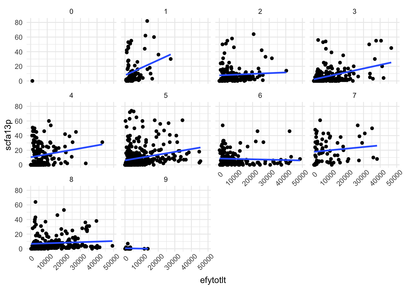

Okay… But what do those variables mean?

Without labels, the plot it hard to understand

So, let’s add labels

The first step is to change facet_wrap(~obereg) to facet_wrap(~as_factor(obereg))
- This is the same as we did in the table above, using a new version of the column that uses the value labels as the value
The second step involves pulling out the variable labels to go on the x and y axis
- This is a little more manual, but, we can set our x and y labels using the labs() argument as normal
  - But instead of putting something like x = "my x axis label", we use the var_label() from the labelled package

ggplot(data |> filter(efytotlt < 50000),
       aes(x = efytotlt,
           y = scfa13p)) +
  geom_point() +
  geom_smooth(method = "lm", se = FALSE) +
  theme_minimal() +
  theme(axis.text.x = element_text(angle = 45, hjust = 0.8)) +
  labs(x = var_label(data$efytotlt),
       y = var_label(data$scfa13p)) +
  facet_wrap(~as_factor(obereg))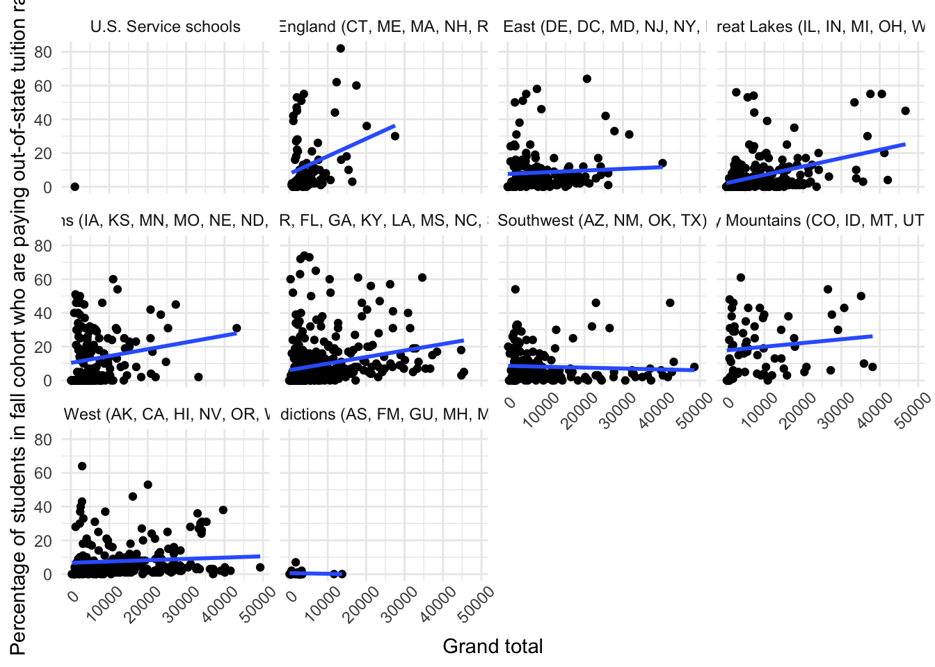

Well, that’s more informative, but a little messy

With a couple of tweaks to allow longer labels to wrap around, we now have a much better looking plot
- y = str_wrap(var_label(data$scfa13p), 40) says to make a new line every 40 characters on the y axis
- labeller = label_wrap_gen(multi_line = TRUE) inside our facet_wrap() allows the facet labels to wrap onto multiple lines

ggplot(data |> filter(efytotlt < 50000),
       aes(x = efytotlt,
           y = scfa13p)) +
  geom_point() +
  geom_smooth(method = "lm", se = FALSE) +
  theme_minimal() +
  theme(axis.text.x = element_text(angle = 45, hjust = 0.8)) +
  labs(x = var_label(data$efytotlt),
       y = str_wrap(var_label(data$scfa13p), 40)) +
  facet_wrap(~as_factor(obereg),
             labeller = label_wrap_gen(multi_line = TRUE))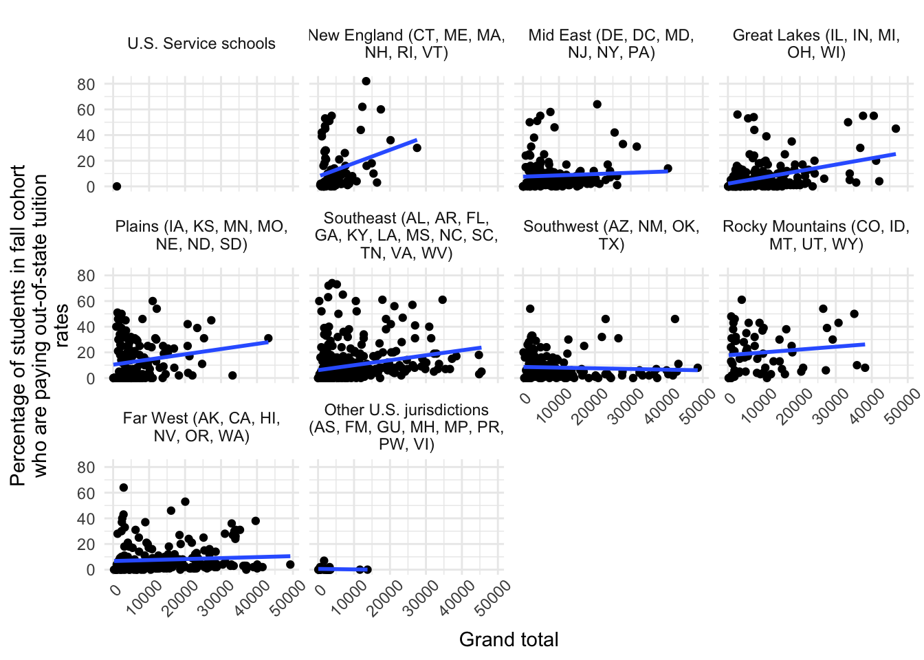

9. What about the relationship between total enrollment and the percent paying instate tuition? Are bigger schools relying more on out-of-state students? Does this trend vary by region?

This wouldn’t work in a table, so, let’s look at a simple scatter plot

scatter scfa13p efytotlt if efytotlt < 50000, by(obereg, col(2))
quietly graph export scatter.svg, replace

See how by default the x, y, and by/facet labels use the labels and not the variable names/values?
- This instantly makes your plots more intuitive
I don’t typically use Stata for plotting, so I’m not sure how to get the longer labels to wrap, but I’m sure there’s a way

5. Models with Labels

R
Stata

11. Lastly, let’s look at how labels can show up in modeling. Let’s see if the percentage of students paying out of state changes by the level of the institution (4 year, 2 year, Less than 2 year)

model <- lm(scfa13p ~ factor(iclevel),
            data = data)

tbl_regression(model)

Characteristic	Beta	95% CI¹	p-value
factor(iclevel)
1	—	—
2	-8.7	-9.9, -7.4	<0.001
3	-14	-21, -7.6	<0.001
¹ CI = Confidence Interval

Without using labels, the regression output needs the code book to interpret

What is iclevel 2?

Remember from above, using as_factor() rather than factor() tells R to use the labels as the levels

model <- lm(scfa13p ~ as_factor(iclevel),
            data = data)

tbl_regression(model)

Characteristic	Beta	95% CI¹	p-value
as_factor(iclevel)
Four or more years	—	—
At least 2 but less than 4 years	-8.7	-9.9, -7.4	<0.001
Less than 2 years (below associate)	-14	-21, -7.6	<0.001
¹ CI = Confidence Interval

Okay that is much clearer what is going on!

as_factor(iclevel) is still a bit messy though
Similarly to the plot above, using variable labels is a little more tricky, but, we can do it using the var_label() function again alongside the label = argument in tbl_regression

tbl_regression(model,
               label = list(`as_factor(iclevel)` = var_label(data$iclevel)))

Characteristic	Beta	95% CI¹	p-value
Level of institution
Four or more years	—	—
At least 2 but less than 4 years	-8.7	-9.9, -7.4	<0.001
Less than 2 years (below associate)	-14	-21, -7.6	<0.001
¹ CI = Confidence Interval

10. Lastly, let’s look at how labels can show up in modeling. Let’s see if the percentage of students paying out of state changes by the level of the institution (4 year, 2 year, Less than 2 year)

regress scfa13p i.iclevel

      Source |       SS           df       MS      Number of obs   =     1,572
-------------+----------------------------------   F(2, 1569)      =     98.14
       Model |  30433.0627         2  15216.5313   Prob > F        =    0.0000
    Residual |  243262.532     1,569  155.043041   R-squared       =    0.1112
-------------+----------------------------------   Adj R-squared   =    0.1101
       Total |  273695.595     1,571  174.217438   Root MSE        =    12.452

-------------------------------------------------------------------------------------
            scfa13p | Coefficient  Std. err.      t    P>|t|     [95% conf. interval]
--------------------+----------------------------------------------------------------
            iclevel |
At least 2 but l..  |  -8.666799   .6320687   -13.71   0.000    -9.906587   -7.427011
Less than 2 yea..)  |  -14.21038    3.35951    -4.23   0.000    -20.79999    -7.62078
                    |
              _cons |   14.21038   .4602254    30.88   0.000     13.30766     15.1131
-------------------------------------------------------------------------------------

As you can see, the variable labels automatically show up in our regression output

Before, you would have seen 2 and 3 in the iclevel column, but now you get informative labels
With the labels, it’s easier to interpret which makes you work easier to read and also less likely you will get mixed up and report the wrong value!

Removing Value Labels

It’s rare, but, there are occasions where you might need to remove value labels from your data

For instance, in R certain advanced analysis packages get confused when you have value labels
You may also spot an error in labelling and need to get rid of it
Luckily, it’s pretty easy!

R
Stata

In R, just use the zap_labels() function from haven to create an unlabelled version of your data

data |>
  count(iclevel)

# A tibble: 3 × 2
  iclevel                                     n
  <dbl+lbl>                               <int>
1 1 [Four or more years]                   2436
2 2 [At least 2 but less than 4 years]     1575
3 3 [Less than 2 years (below associate)]  1669

data_unlabelled <- zap_labels(data)

data_unlabelled |>
  count(iclevel)

# A tibble: 3 × 2
  iclevel     n
    <dbl> <int>
1       1  2436
2       2  1575
3       3  1669

In Stata, simply type label drop _all

tabulate iclevel

label drop _all

tabulate iclevel

               Level of institution |      Freq.     Percent        Cum.
------------------------------------+-----------------------------------
                 Four or more years |      2,436       42.89       42.89
   At least 2 but less than 4 years |      1,575       27.73       70.62
Less than 2 years (below associate) |      1,669       29.38      100.00
------------------------------------+-----------------------------------
                              Total |      5,680      100.00



   Level of |
institution |      Freq.     Percent        Cum.
------------+-----------------------------------
          1 |      2,436       42.89       42.89
          2 |      1,575       27.73       70.62
          3 |      1,669       29.38      100.00
------------+-----------------------------------
      Total |      5,680      100.00

Getting Capitalized Variable Names

By default, IPEDtaS gives you lower-case variable names (which is the default for Stata-style data)
Usually, this is going to be easier to work with
- However, sometimes you might need to keep the original upper-case variable names, such as if you’re adding this to an existing project that already uses upper-case variable names
To do this, you just need to add a single line near the end of the IPEDtaS script

R
Stata

Add this line

data_file <- data_file |> dplyr::rename_all(stringr::str_to_upper)

directly above (near end of script)

haven::write_dta(data_file, dta_name)