II: Appending, joining, & reshaping data

So far, we have only worked with single data files: we read in a file, wrangled our data, and, sometimes, outputted a new file.
But very often, a key aspect of the data wrangling workflow is to combine more than one data set together. This may include;
- appending new rows to an existing data frame in memory
- joining two data sets together using a common key value found in both.
As part of this, we often will need to;
- reshape our data, pivoting from wide to long form (or vice versa).
We’ll go through each individually below.

Data

The data for today’s lesson is all in your data/sch-test folder
- It should look something like this:

|__ data/
    |-- ...
    |__ sch_test/
        |-- all_schools.csv
        |-- all_schools_wide.csv
        |__ by_school/
            |-- bend_gate_1980.csv
            |-- bend_gate_1981.csv
            |...
            |-- spottsville_1985.csv

These fake data represent test scores across three subjects — math, reading, and science — across four schools over six years.
Each school has a file for each year in the by_school subdirectory.
The two files in sch_test directory, all_schools.csv and all_schools_wide.csv, combine the individual files but in different formats.
- We’ll use these data sets to practice appending, joining, and reshaping.

Setup

As always, we begin by reading in the tidyverse library.

## ---------------------------
##' [Libraries]
## ---------------------------

library(tidyverse)

As we did in the past lesson, we will run this script assuming that our working directory is set to the project folder

Appending data

Our first task is the most straightforward. When appending data, we simply add similarly structured rows to an exiting data frame.
What is similarly structured? Imagine you have a data frame that looks like this:

id	year	score
A	2020	98
B	2020	95
C	2020	85
D	2020	94

Now, assume you are given data that look like this:

id	year	score
E	2020	99
F	2020	90

These data are similarly structured: same column names in the same order. If we know that the data came from the same process (e.g., ids represent students in the same classroom with each file representing a different test day), then we can safely append the second to the first:

id	year	score
A	2020	98
B	2020	95
C	2020	85
D	2020	94
E	2020	99
F	2020	90

Data that are the result of the exact same data collecting process across locations or time may be appended. In education research, administrative data are often recorded each term or year, meaning you can build a panel data set by appending. The NCES IPEDS data files generally work like this
- Note on IPEDS: Some of the variables have changed over time, one of the most notable being enrollment data between 2001 and 2002, so always check your dictionary (codebook)!
However, it’s incumbent upon you as the researcher to understand your data. Just because you are able to append (R will try to make it work for you) doesn’t mean you always should.
- What if the score column in our data weren’t on the same scale?
- What if the test date mattered but isn’t included in the file?
- What if the files actually represent scores from different grades or schools?
It’s possible that we can account for each of these issues as we clean our data, but it won’t happen automatically — append with care!

Example

Let’s practice with an example. First, we’ll read in three data files from the by_school directory.

## read in data, storing in data_*, where * is a unique number
data_1 <- read_csv("data/sch-test/by-school/bend-gate-1980.csv")
data_2 <- read_csv("data/sch-test/by-school/bend-gate-1981.csv")
data_3 <- read_csv("data/sch-test/by-school/bend-gate-1982.csv")

Looking at each, we can see that they are similarly structured, with the following columns in the same order: school, year, math, read, science:

## show each
data_1

# A tibble: 1 × 5
  school     year  math  read science
  <chr>     <dbl> <dbl> <dbl>   <dbl>
1 Bend Gate  1980   515   281     808

data_2

# A tibble: 1 × 5
  school     year  math  read science
  <chr>     <dbl> <dbl> <dbl>   <dbl>
1 Bend Gate  1981   503   312     814

data_3

# A tibble: 1 × 5
  school     year  math  read science
  <chr>     <dbl> <dbl> <dbl>   <dbl>
1 Bend Gate  1982   514   316     816

From the dplyr library, we use the bind_rows() function to append the second and third data frames to the first.

## append files
data <- bind_rows(data_1, data_2, data_3)

## show
data

# A tibble: 3 × 5
  school     year  math  read science
  <chr>     <dbl> <dbl> <dbl>   <dbl>
1 Bend Gate  1980   515   281     808
2 Bend Gate  1981   503   312     814
3 Bend Gate  1982   514   316     816

That’s it!

Quick exercise

Read in the rest of the files for Bend Gate and append them to the current data frame.

Quick exercise: Take Two

If bind_rows() stacks tables on top of each other, what do you think would stack them side-by-side? Copy the below code and try to figure how to get them back together

data_split_left <- data[,1:2]
data_split_right <- data[,3:5]

print(data_split_left)

# A tibble: 3 × 2
  school     year
  <chr>     <dbl>
1 Bend Gate  1980
2 Bend Gate  1981
3 Bend Gate  1982

print(data_split_right)

# A tibble: 3 × 3
   math  read science
  <dbl> <dbl>   <dbl>
1   515   281     808
2   503   312     814
3   514   316     816

## Append them back together side-by-side

Joining data

More often than appending your data files, however, you will need to merge or join them.
With a join, you add to your data frame new columns (new variables) that come from a second data frame.
The key difference between joining and appending is that a join requires a key, that is, a variable or index common to each data frame that uniquely identifies observations.
- It’s this key that’s used to line everything up.

For example, say you have these two data sets,

id	sch	year	score
A	1	2020	98
B	1	2020	95
C	2	2020	85
D	3	2020	94

sch	type
1	elementary
2	middle
3	high

You want to add the school type to the first data set.
You can do this because you have a common key between each set: sch.

Add a column to the first data frame called type
Fill in each row of the new column with the type value that corresponds to the matching sch value in both data frames:
- sch == 1 --> elementary
- sch == 2 --> middle
- sch == 3 --> high

The end result would then look like this:

id	sch	year	score	type
A	1	2020	98	elementary
B	1	2020	95	elementary
C	2	2020	85	middle
D	3	2020	94	high

Example

A common join task in education research involves adding group-level aggregate statistics to individual observations, for example;
- adding school-level average test scores to each student’s row.
- With a panel data set (observations across time), we might want within-year averages added to each unit-by-time period row.
Let’s do the second, adding within-year across school average test scores to each school-by-year observation.

## read in all_schools data
data <- read_csv("data/sch-test/all-schools.csv")

Looking at the data, we see that it’s similar to what we’ve seen above, with additional schools.

## show
data

# A tibble: 24 × 5
   school        year  math  read science
   <chr>        <dbl> <dbl> <dbl>   <dbl>
 1 Bend Gate     1980   515   281     808
 2 Bend Gate     1981   503   312     814
 3 Bend Gate     1982   514   316     816
 4 Bend Gate     1983   491   276     793
 5 Bend Gate     1984   502   310     788
 6 Bend Gate     1985   488   280     789
 7 East Heights  1980   501   318     782
 8 East Heights  1981   487   323     813
 9 East Heights  1982   496   294     818
10 East Heights  1983   497   306     795
# ℹ 14 more rows

Our task is two-fold:

Get the average of each test score (math, reading, science) across all schools within each year and save the summary data frame in an object.
Join the new summary data frame to the original data frame.

1. Get summary

## get test score summary 
data_sum <- data |>
    ## grouping by year so average within each year
    group_by(year) |>
    ## get mean(<score>) for each test
    summarize(math_m = mean(math),
              read_m = mean(read),
              science_m = mean(science))

## show
data_sum

# A tibble: 6 × 4
   year math_m read_m science_m
  <dbl>  <dbl>  <dbl>     <dbl>
1  1980   507    295.      798.
2  1981   496.   293.      788.
3  1982   506    302.      802.
4  1983   500    293.      794.
5  1984   490    300.      792.
6  1985   500.   290.      794.

Quick exercise

Thinking ahead, why do you think we created new names for the summarized columns? Why the _m ending?

2. Join

While one can merge using base R, dplyr (part of the tidyverse package) is what we will be using in this lesson.
Here are the most common joins you will use:
left_join(x, y, by = ): keep all x, drop unmatched y
right_join(x, y, by = ): keep all y, drop unmatched x
inner_join(x, y, by = ): keep only matching
full_join(x, y, by = ): keep everything
anti_join(x, y, by = ): keep only obs in x and that are not in y (more useful than you’d think)
Essentially, all _join() functions takes three main “arguments” and they have always the same meaning
- x data one, a.k.a. the “left” data
- y data two, a.k.a. the “right” data
- by the variables to use as a “key”

`by`

Whichever type of _join you are doing, the by argument is just how x and y are being matched up
- by has to be at least one variable that is in both x and y and identifies the same observation
  - e.g., by = "school_id"
  - Most often this will be some kind of identifying variable (student ID, school ID, city, state, region, etc.)
- If have more than one piece of information to match on, such as school and year, we can specify that with c()
  - e.g., by = c("school_id", "year")
  - This will then find information for each school in each year, and join it in correctly
If you don’t provide any by arguments, R will try to be smart and look for columns names that are the same in both data sets
- This can lead to incorrect joins though, so always best to specify
Lastly, if you need to join by columns that have different names in each data set use c("name in df_1" = "name in df_2")
- e.g., by = c("student_id" = "id_number")

Conceptual example

For example, the result of a left join between data frame X and data frame Y will include all observations in X and those in Y that are also in X.

id	col_A	col_B
001	a	1
002	b	2
003	a	3

id	col_C	col_D
001	T	9
002	T	9
004	F	9

XY (result of left join)

id	col_A	col_B	col_C	col_D
001	a	1	T	9
002	b	2	T	9
003	a	3	NA	NA

Observations in both X and Y (001 and 002, above), will have data for the columns that were separately in X and Y before.
Those in X only (003), will have missing values in the new columns that came from Y because they didn’t exist there.
Observations in Y but not X (004) are dropped entirely.

Practice joining

Back to our example…

Since we want to join a smaller aggregated data frame, df_sum, to the original data frame, df, we’ll use a left_join().
- The join functions will try to guess the joining variable (and tell you what it picked) if you don’t supply one, but we’ll specify one to be clear.

## start with our dataframe...
data_joined <- data |>
    ## pipe into left_join to join with data_sum using "year" as key
    left_join(data_sum, by = "year")

## show
data_joined

# A tibble: 24 × 8
   school        year  math  read science math_m read_m science_m
   <chr>        <dbl> <dbl> <dbl>   <dbl>  <dbl>  <dbl>     <dbl>
 1 Bend Gate     1980   515   281     808   507    295.      798.
 2 Bend Gate     1981   503   312     814   496.   293.      788.
 3 Bend Gate     1982   514   316     816   506    302.      802.
 4 Bend Gate     1983   491   276     793   500    293.      794.
 5 Bend Gate     1984   502   310     788   490    300.      792.
 6 Bend Gate     1985   488   280     789   500.   290.      794.
 7 East Heights  1980   501   318     782   507    295.      798.
 8 East Heights  1981   487   323     813   496.   293.      788.
 9 East Heights  1982   496   294     818   506    302.      802.
10 East Heights  1983   497   306     795   500    293.      794.
# ℹ 14 more rows

Quick exercise

Look at the first 10 rows of data_joined. What do you notice about the new summary columns we added?

Using the `|>` pipe

Now, if you remember from Data Wrangling I, the |> makes R code more intuitive by “piping” one thing into the next
- This makes things simpler 99% of the time (no one wants to be writing nested code)
- But in this case it takes a second to get your head around
By default, the pipe |> will always go into the first “argument” of a function, which in this case, is x
- We can always specify where it should go with an _ underscore

## Therefore 
left_join(x = data,
          y = data_sum,
          by = "year")

# A tibble: 24 × 8
   school        year  math  read science math_m read_m science_m
   <chr>        <dbl> <dbl> <dbl>   <dbl>  <dbl>  <dbl>     <dbl>
 1 Bend Gate     1980   515   281     808   507    295.      798.
 2 Bend Gate     1981   503   312     814   496.   293.      788.
 3 Bend Gate     1982   514   316     816   506    302.      802.
 4 Bend Gate     1983   491   276     793   500    293.      794.
 5 Bend Gate     1984   502   310     788   490    300.      792.
 6 Bend Gate     1985   488   280     789   500.   290.      794.
 7 East Heights  1980   501   318     782   507    295.      798.
 8 East Heights  1981   487   323     813   496.   293.      788.
 9 East Heights  1982   496   294     818   506    302.      802.
10 East Heights  1983   497   306     795   500    293.      794.
# ℹ 14 more rows

## Is exactly the same as
data |>
  left_join(x = _, ## If it helps to visualize, the _ is where the |> will go
            y = data_sum,
            by = "year")

# A tibble: 24 × 8
   school        year  math  read science math_m read_m science_m
   <chr>        <dbl> <dbl> <dbl>   <dbl>  <dbl>  <dbl>     <dbl>
 1 Bend Gate     1980   515   281     808   507    295.      798.
 2 Bend Gate     1981   503   312     814   496.   293.      788.
 3 Bend Gate     1982   514   316     816   506    302.      802.
 4 Bend Gate     1983   491   276     793   500    293.      794.
 5 Bend Gate     1984   502   310     788   490    300.      792.
 6 Bend Gate     1985   488   280     789   500.   290.      794.
 7 East Heights  1980   501   318     782   507    295.      798.
 8 East Heights  1981   487   323     813   496.   293.      788.
 9 East Heights  1982   496   294     818   506    302.      802.
10 East Heights  1983   497   306     795   500    293.      794.
# ℹ 14 more rows

## Is exactly the same as
data |>
  left_join(data_sum,
            by = "year")

# A tibble: 24 × 8
   school        year  math  read science math_m read_m science_m
   <chr>        <dbl> <dbl> <dbl>   <dbl>  <dbl>  <dbl>     <dbl>
 1 Bend Gate     1980   515   281     808   507    295.      798.
 2 Bend Gate     1981   503   312     814   496.   293.      788.
 3 Bend Gate     1982   514   316     816   506    302.      802.
 4 Bend Gate     1983   491   276     793   500    293.      794.
 5 Bend Gate     1984   502   310     788   490    300.      792.
 6 Bend Gate     1985   488   280     789   500.   290.      794.
 7 East Heights  1980   501   318     782   507    295.      798.
 8 East Heights  1981   487   323     813   496.   293.      788.
 9 East Heights  1982   496   294     818   506    302.      802.
10 East Heights  1983   497   306     795   500    293.      794.
# ℹ 14 more rows

You can write joins whichever way you want (piped or not-piped)
- Eventually, you will find piped is easier and more-efficient, but focus on whichever way makes more sense to you for now

## Note: if we want to keep the joined data, we should assign it to df_join
data_join <- data |>
  left_join(data_sum,
            by = "year")

`_join` summary

Joining data is one of the most important tasks in educational research
- IPEDS Complete Data Files are the perfect example, within each year all the data is stored in separate files that need joining
  - Remember the same IPEDS files for different years need bind_rows() once you add a year identifier
It takes a while to get your head around, but if you can do it properly, you are well on the way to mastering data wrangling!

Reshaping data

Reshaping data is a common and important data wrangling task.
Whether going from wide to long format or long to wide, it can be a painful process.
- But with a little practice, the ability to reshape data will become a powerful tool in your toolbox.

Definitions

While there are various definitions of tabular data structure, the two you will most often come across are wide and long.
- Wide data are data structures in which all variable/values are columns.
  - At the extreme end, every id will only have a single row:

id	math_score_2019	read_score_2019	math_score_2020	read_score_2020
A	93	88	92	98
B	99	92	97	95
C	89	88	84	85

Notice how each particular score (by year) has its own column?
- Compare this to long data in which each observational unit (id test score within a given year) will have a row:

id	year	test	score
A	2019	math	93
A	2019	read	88
A	2020	math	92
A	2020	read	98
B	2019	math	99
B	2019	read	92
B	2020	math	97
B	2020	read	95
C	2019	math	89
C	2019	read	88
C	2020	math	84
C	2020	read	85

The first wide and second long table present the same information in a different format.
- So why bother reshaping?
  - The short answer is that you sometimes need one format and sometimes the other due to the demands of the analysis you want to run, the figure you want to plot, or the table you want to make.

Note: Data in the wild are often some combination of these two types: wide-ish or long-ish. For an example, see our all-schools.csv data below, which is wide in some variables (test), but long in others (year). The point of defining long vs wide is not to have a testable definition, but rather to have a framework for thinking about how your data are structured and if that structure will work for your data analysis needs.

Example: wide –> long

To start, we’ll go back to the all_schools.csv file.

## reading again just to be sure we have the original data
data <- read_csv("data/sch-test/all-schools.csv")

## print to see what the data structure looks like
print(data)

# A tibble: 24 × 5
   school        year  math  read science
   <chr>        <dbl> <dbl> <dbl>   <dbl>
 1 Bend Gate     1980   515   281     808
 2 Bend Gate     1981   503   312     814
 3 Bend Gate     1982   514   316     816
 4 Bend Gate     1983   491   276     793
 5 Bend Gate     1984   502   310     788
 6 Bend Gate     1985   488   280     789
 7 East Heights  1980   501   318     782
 8 East Heights  1981   487   323     813
 9 East Heights  1982   496   294     818
10 East Heights  1983   497   306     795
# ℹ 14 more rows

Notice how the data are wide in test:
- Each school has one row per year, but each test (math, read, science) gets its own column.
- While this setup can be efficient for storage, it’s not always the best for analysis or even just browsing.
  - What we want is for the data to be long.
Instead of each test having its own column, we would like to make the data look like our long data example above, with each row representing a single school, year, test, score:

school	year	test	score
Bend Gate	1980	math	515
Bend Gate	1980	read	281
Bend Gate	1980	science	808
…	…	…	…

As with joins, you can reshape data frames using base R commands.
But again, we’ll use tidyverse functions in the tidyr library.
- Specifically, we’ll rely on the tidyr pivot_longer() and pivot_wider() commands.

`pivot_longer()`

The pivot_longer() function can take a number of arguments, but the core things it needs to know are:

data: the name of the data frame you’re reshaping (we can use |> to pipe in the data name)
cols: the names of the columns that you want to pivot into values of a single new column (thereby making the data frame “longer”)
names_to: the name of the new column that will contain the names of the cols you just listed
values_to: the name of the column where the values in the cols you listed will go
In our current situation, our cols to pivot are "math", "read", and "science".
- Since they are test types, we’ll call our names_to column "test" and our values_to column "score".

## wide to long
data_long <- data |>
    ## cols: current test columns
    ## names_to: where "math", "read", and "science" will go
    ## values_to: where the values in cols will go
    pivot_longer(cols = c("math","read","science"),
                 names_to = "test",
                 values_to = "score")

## show
data_long

# A tibble: 72 × 4
   school     year test    score
   <chr>     <dbl> <chr>   <dbl>
 1 Bend Gate  1980 math      515
 2 Bend Gate  1980 read      281
 3 Bend Gate  1980 science   808
 4 Bend Gate  1981 math      503
 5 Bend Gate  1981 read      312
 6 Bend Gate  1981 science   814
 7 Bend Gate  1982 math      514
 8 Bend Gate  1982 read      316
 9 Bend Gate  1982 science   816
10 Bend Gate  1983 math      491
# ℹ 62 more rows

Quick (ocular test) exercise

How many rows did our initial data frame df have? How many unique tests did we have in each year? When reshaping from wide to long, how many rows should we expect our new data frame to have? Does our new data frame have that many rows?

Example: long –> wide

`pivot_wider()`

Now that we have our long data, let’s reshape it back to wide format using pivot_wider(). In this case, we’re doing just the opposite from before — here are the main arguments you need to attend to:
data: the name of the data frame you’re reshaping (we can use |> to pipe in the data name)
names_from: the name of the column that contains the values which will become new column names
values_from: the name of the column that contains the values associated with the values in names_from column; these will go into the new columns.

## long to wide
data_wide <- data_long |>
    ## names_from: values in this column will become new column names
    ## values_from: values in this column will become values in new cols
    pivot_wider(names_from = "test",
                values_from = "score")

## show
data_wide

# A tibble: 24 × 5
   school        year  math  read science
   <chr>        <dbl> <dbl> <dbl>   <dbl>
 1 Bend Gate     1980   515   281     808
 2 Bend Gate     1981   503   312     814
 3 Bend Gate     1982   514   316     816
 4 Bend Gate     1983   491   276     793
 5 Bend Gate     1984   502   310     788
 6 Bend Gate     1985   488   280     789
 7 East Heights  1980   501   318     782
 8 East Heights  1981   487   323     813
 9 East Heights  1982   496   294     818
10 East Heights  1983   497   306     795
# ℹ 14 more rows

`pivot_()`-ing with separation

Unfortunately, it’s not always so clear cut to reshape data.
In this second example, we’ll again reshape from wide to long, but with an extra argument that helps when there’s more than one piece of information in the variable name

First, we’ll read in a second file all_schools_wide.csv - This file contains the same information as before, but in a very wide format

## read in very wide test score data
data <- read_csv("data/sch-test/all-schools-wide.csv")

## show
data

# A tibble: 4 × 19
  school       math_1980 read_1980 science_1980 math_1981 read_1981 science_1981
  <chr>            <dbl>     <dbl>        <dbl>     <dbl>     <dbl>        <dbl>
1 Bend Gate          515       281          808       503       312          814
2 East Heights       501       318          782       487       323          813
3 Niagara            514       292          787       499       268          762
4 Spottsville        498       288          813       494       270          765
# ℹ 12 more variables: math_1982 <dbl>, read_1982 <dbl>, science_1982 <dbl>,
#   math_1983 <dbl>, read_1983 <dbl>, science_1983 <dbl>, math_1984 <dbl>,
#   read_1984 <dbl>, science_1984 <dbl>, math_1985 <dbl>, read_1985 <dbl>,
#   science_1985 <dbl>

You see, each school has only one row and each test by year value gets its own column in the form <test>_<year>.

We will use pivot_longer() just as we did before
- But instead of one column for names_to we use our friend c() to list two columns we want the information from column name to go to
- Then, we add names_sep = "_", which means separate the information from the names at every underscore
  - I.e., this will put everything before the underscore in the first column test and everything after into the second column year

## wide to long
data_long <- data |>
    ## contains() looks for "19" in name: if there, it adds it to cols
    pivot_longer(cols = contains("19"),
                 names_to = c("test", "year"),
                 names_sep = "_",
                 values_to = "score")

## show
data_long

# A tibble: 72 × 4
   school    test    year  score
   <chr>     <chr>   <chr> <dbl>
 1 Bend Gate math    1980    515
 2 Bend Gate read    1980    281
 3 Bend Gate science 1980    808
 4 Bend Gate math    1981    503
 5 Bend Gate read    1981    312
 6 Bend Gate science 1981    814
 7 Bend Gate math    1982    514
 8 Bend Gate read    1982    316
 9 Bend Gate science 1982    816
10 Bend Gate math    1983    491
# ℹ 62 more rows

Quick exercise(s)

What do you think we’d need to change if the column name had 3 pieces of information all separated by an underscore?

What about if the information was separated by a . period?

Now, if we want to get our data back in to extra long form, we can use a very similar argument in pivot_wider()
- We just use c() to say get the name information from two columns
- names_sep = "_" is identical to before, but this time it’s saying to place and underscore as the separator

## wide to long
data_wide <- data_long |>
    pivot_wider(values_from = score,
                names_from = c(test, year),
                names_sep = "_")

## show
data_wide

# A tibble: 4 × 19
  school       math_1980 read_1980 science_1980 math_1981 read_1981 science_1981
  <chr>            <dbl>     <dbl>        <dbl>     <dbl>     <dbl>        <dbl>
1 Bend Gate          515       281          808       503       312          814
2 East Heights       501       318          782       487       323          813
3 Niagara            514       292          787       499       268          762
4 Spottsville        498       288          813       494       270          765
# ℹ 12 more variables: math_1982 <dbl>, read_1982 <dbl>, science_1982 <dbl>,
#   math_1983 <dbl>, read_1983 <dbl>, science_1983 <dbl>, math_1984 <dbl>,
#   read_1984 <dbl>, science_1984 <dbl>, math_1985 <dbl>, read_1985 <dbl>,
#   science_1985 <dbl>

Final note

Just as all data sets are unique, so too are the particular steps you may need to take to append, join, or reshape your data.
- Even experienced coders rarely get all the steps correct the first try.
- Be prepared to spend time getting to know your data and figuring out, through trial and error, how to wrangle it so that it meets your analytic needs.
- Code books, institutional/domain knowledge, and patience are your friends here!

Now, let’s look at a more realistic example when we would use these skills for data analysis
Let’s say we want to explore difference in international student enrollment at the undergraduate vs graduate level and if that varies by region of the US
For this, we are going to use two IPEDS data sets HD2022 and EFFY2022
- Note: These data sets are not in your class repository (intentionally), so we have to go and download them from the IPEDS Data Center

data_info <- read_csv("data/hd2022.csv")
data_enroll <- read_csv("data/effy2022.csv")

Let’s take a look at these data one by one

data_info

# A tibble: 6,256 × 73
   UNITID INSTNM     IALIAS ADDR  CITY  STABBR ZIP    FIPS OBEREG CHFNM CHFTITLE
    <dbl> <chr>      <chr>  <chr> <chr> <chr>  <chr> <dbl>  <dbl> <chr> <chr>   
 1 100654 Alabama A… AAMU   4900… Norm… AL     35762     1      5 Dr. … Preside…
 2 100663 Universit… UAB    Admi… Birm… AL     3529…     1      5 Ray … Preside…
 3 100690 Amridge U… South… 1200… Mont… AL     3611…     1      5 Mich… Preside…
 4 100706 Universit… UAH  … 301 … Hunt… AL     35899     1      5 Chuc… Preside…
 5 100724 Alabama S… <NA>   915 … Mont… AL     3610…     1      5 Quin… Preside…
 6 100733 Universit… <NA>   500 … Tusc… AL     35401     1      5 Fini… Chancel…
 7 100751 The Unive… <NA>   739 … Tusc… AL     3548…     1      5 Dr. … Preside…
 8 100760 Central A… <NA>   1675… Alex… AL     35010     1      5 Jeff… Preside…
 9 100812 Athens St… <NA>   300 … Athe… AL     35611     1      5 Dr. … Interim…
10 100830 Auburn Un… AUM||… 7440… Mont… AL     3611…     1      5 Carl… Chancel…
# ℹ 6,246 more rows
# ℹ 62 more variables: GENTELE <dbl>, EIN <chr>, UEIS <chr>, OPEID <chr>,
#   OPEFLAG <dbl>, WEBADDR <chr>, ADMINURL <chr>, FAIDURL <chr>, APPLURL <chr>,
#   NPRICURL <chr>, VETURL <chr>, ATHURL <chr>, DISAURL <chr>, SECTOR <dbl>,
#   ICLEVEL <dbl>, CONTROL <dbl>, HLOFFER <dbl>, UGOFFER <dbl>, GROFFER <dbl>,
#   HDEGOFR1 <dbl>, DEGGRANT <dbl>, HBCU <dbl>, HOSPITAL <dbl>, MEDICAL <dbl>,
#   TRIBAL <dbl>, LOCALE <dbl>, OPENPUBL <dbl>, ACT <chr>, NEWID <dbl>, …

Okay, this looks simple enough, we see one row per institution followed by a bunch of descriptive variables
Let’s look at our enrollment data

data_enroll

# A tibble: 117,521 × 72
   UNITID EFFYALEV EFFYLEV LSTUDY XEYTOTLT EFYTOTLT XEYTOTLM EFYTOTLM XEYTOTLW
    <dbl>    <dbl>   <dbl>  <dbl> <chr>       <dbl> <chr>       <dbl> <chr>   
 1 100654        1       1    999 R            6681 R            2666 R       
 2 100654        2       2      1 R            5663 R            2337 R       
 3 100654        3      -2      1 R            5621 R            2323 R       
 4 100654        4      -2      1 R            1680 R             722 R       
 5 100654        5      -2      1 R            3941 R            1601 R       
 6 100654       11      -2      1 R              42 R              14 R       
 7 100654       12       4      3 R            1018 R             329 R       
 8 100654       19      -2      1 R             361 R             177 R       
 9 100654       20      -2      1 R            3580 R            1424 R       
10 100654       21      -2    999 R            5460 R            2169 R       
# ℹ 117,511 more rows
# ℹ 63 more variables: EFYTOTLW <dbl>, XEFYAIAT <chr>, EFYAIANT <dbl>,
#   XEFYAIAM <chr>, EFYAIANM <dbl>, XEFYAIAW <chr>, EFYAIANW <dbl>,
#   XEFYASIT <chr>, EFYASIAT <dbl>, XEFYASIM <chr>, EFYASIAM <dbl>,
#   XEFYASIW <chr>, EFYASIAW <dbl>, XEFYBKAT <chr>, EFYBKAAT <dbl>,
#   XEFYBKAM <chr>, EFYBKAAM <dbl>, XEFYBKAW <chr>, EFYBKAAW <dbl>,
#   XEFYHIST <chr>, EFYHISPT <dbl>, XEFYHISM <chr>, EFYHISPM <dbl>, …

Hmm, so this data definitely appears to be “long” as we see those first 10 rows are all for 100654
- Based on visual inspection, it seems like EFFYALEV and EFFYLEV might be what is making the data “long” for two reasons
  - First, look at the values, they seem seem to increasing in some kind of pattern
  - Second, it’s common practice to keep the “long” variables at the start, especially in larger published data like this
- This is where we want to look through the code book to explore what those variables might mean

Quick Exercise

To practice this, let’s go to the IPEDS Data Center and find the dictionary for EFFY2022

Tip: For IPEDS dictionary files, the “frequencies” tab is where you’ll find out what numbers that represent something mean

Okay, so what so EFFYALEV and EFFYLEV mean?

Think back to our research question, what’s the ratio of international students at the undergraduate vs graduate level?

Based on the code book, what do you think we need to do now?

EFFYALEV is probably more detail than we need for our question, EFFYLEV has everything we need
- To make our life simpler, let’s reduce our data down a little to just the variables we want with select()

data_enroll <- data_enroll |>
  select(UNITID, EFFYLEV, EFYTOTLT, EFYNRALT)

data_enroll

# A tibble: 117,521 × 4
   UNITID EFFYLEV EFYTOTLT EFYNRALT
    <dbl>   <dbl>    <dbl>    <dbl>
 1 100654       1     6681      104
 2 100654       2     5663       53
 3 100654      -2     5621       53
 4 100654      -2     1680       12
 5 100654      -2     3941       41
 6 100654      -2       42        0
 7 100654       4     1018       51
 8 100654      -2      361       10
 9 100654      -2     3580       31
10 100654      -2     5460       95
# ℹ 117,511 more rows

Next, let’s reduce our data down to just the two rows containing undergraduate and graduate enrollments

data_enroll <- data_enroll |>
  filter(EFFYLEV %in% c(2,4))
  
data_enroll

# A tibble: 7,817 × 4
   UNITID EFFYLEV EFYTOTLT EFYNRALT
    <dbl>   <dbl>    <dbl>    <dbl>
 1 100654       2     5663       53
 2 100654       4     1018       51
 3 100663       2    15360      415
 4 100663       4    10603     1047
 5 100690       2      351        0
 6 100690       4      565        0
 7 100706       2     8536      187
 8 100706       4     2606      234
 9 100724       2     3899       60
10 100724       4      526        8
# ℹ 7,807 more rows

Okay, this is starting to look more manageable, right?
What do we need to do next to be able to compare across levels of study or institutions?

data_enroll <- data_enroll |>
  mutate(perc_intl = EFYNRALT/EFYTOTLT*100) |>
  select(-EFYTOTLT, -EFYNRALT) # - in select means drop this variable

data_enroll

# A tibble: 7,817 × 3
   UNITID EFFYLEV perc_intl
    <dbl>   <dbl>     <dbl>
 1 100654       2     0.936
 2 100654       4     5.01 
 3 100663       2     2.70 
 4 100663       4     9.87 
 5 100690       2     0    
 6 100690       4     0    
 7 100706       2     2.19 
 8 100706       4     8.98 
 9 100724       2     1.54 
10 100724       4     1.52 
# ℹ 7,807 more rows

Now, we want to find the difference between the undergraduate and graduate enrollment levels, which should be pretty simple math right? We just need to subtract the percentages from each other
- Can we easily do that right now? If not, what do we need to do?

data_enroll <- data_enroll |>
  pivot_wider(names_from = EFFYLEV,
              values_from = perc_intl,
              names_prefix = "perc_intl_")

data_enroll

# A tibble: 6,036 × 3
   UNITID perc_intl_2 perc_intl_4
    <dbl>       <dbl>       <dbl>
 1 100654      0.936         5.01
 2 100663      2.70          9.87
 3 100690      0             0   
 4 100706      2.19          8.98
 5 100724      1.54          1.52
 6 100751      1.62         10.7 
 7 100760      0.406        NA   
 8 100812      0.0577        0   
 9 100830      4.32         37.5 
10 100858      4.42         17.7 
# ℹ 6,026 more rows

Now is our calculation much easier to make?

data_enroll <- data_enroll |>
  mutate(perc_intl_diff = perc_intl_2 - perc_intl_4)

data_enroll

# A tibble: 6,036 × 4
   UNITID perc_intl_2 perc_intl_4 perc_intl_diff
    <dbl>       <dbl>       <dbl>          <dbl>
 1 100654      0.936         5.01        -4.07  
 2 100663      2.70          9.87        -7.17  
 3 100690      0             0            0     
 4 100706      2.19          8.98        -6.79  
 5 100724      1.54          1.52         0.0179
 6 100751      1.62         10.7         -9.04  
 7 100760      0.406        NA           NA     
 8 100812      0.0577        0            0.0577
 9 100830      4.32         37.5        -33.2   
10 100858      4.42         17.7        -13.3   
# ℹ 6,026 more rows

How do we interpret our new variable?
Let’s get some basic summary statistics

data_enroll |>
  drop_na() |>
  summarize(mean = mean(perc_intl_diff),
            min = min(perc_intl_diff),
            max = max(perc_intl_diff))

# A tibble: 1 × 3
   mean   min   max
  <dbl> <dbl> <dbl>
1 -3.84 -96.8  41.5

Lastly, let’s see if this trend varies by private vs public institutions
What do we need to do to see that?

data_info <- data_info |>
  select(UNITID, CONTROL)

data_joined <- left_join(data_enroll, data_info, by = "UNITID")

data_joined

# A tibble: 6,036 × 5
   UNITID perc_intl_2 perc_intl_4 perc_intl_diff CONTROL
    <dbl>       <dbl>       <dbl>          <dbl>   <dbl>
 1 100654      0.936         5.01        -4.07         1
 2 100663      2.70          9.87        -7.17         1
 3 100690      0             0            0            2
 4 100706      2.19          8.98        -6.79         1
 5 100724      1.54          1.52         0.0179       1
 6 100751      1.62         10.7         -9.04         1
 7 100760      0.406        NA           NA            1
 8 100812      0.0577        0            0.0577       1
 9 100830      4.32         37.5        -33.2          1
10 100858      4.42         17.7        -13.3          1
# ℹ 6,026 more rows

Looks like we have what we need, so let’s see if the mean varies by institutional control

data_joined |>
  group_by(CONTROL) |>
  drop_na() |>
  summarize(mean = mean(perc_intl_diff))

# A tibble: 3 × 2
  CONTROL  mean
    <dbl> <dbl>
1       1 -5.84
2       2 -2.63
3       3 -4.94

Quick Exercise

Using the data dictionary if necessary, find if our trend varies by US Census Region

Assignment Template

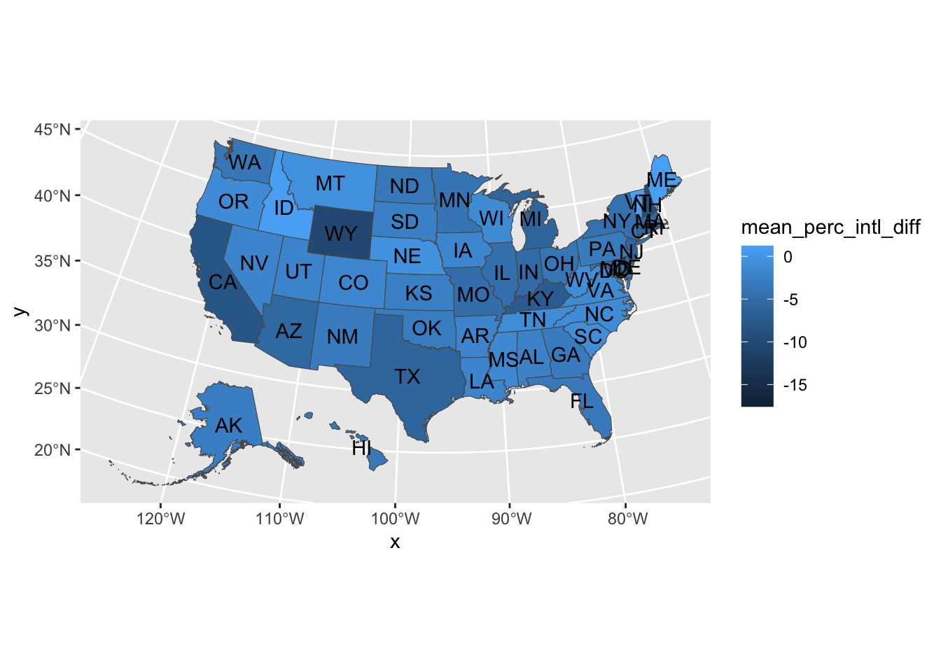
Use the hsls_small.csv data set from the lesson answer the following questions

Throughout, you should account for missing values by dropping them

Hint: You’re going to need the code book to identify the necessary variables

Question One

a) Compute the average test score by region

b) Join back into the full data frame

c) Compute the difference between each student’s test score and that of the region

d) Finally, show the mean of these differences by region

Hint: If you think about it, this should probably be a very very small number…

e) Optional: Do all of the above steps in one piped chain of commands

Question Two

a) Compute the average test score by region and family income level

b) Join that average score back to the full data frame

Hint: You can join on more than one key using c()

c) Optional: Do all of the above steps in one piped chain of commands

Question Three

a) Select the following variables from the full data set

stu_id
x1stuedexpct
x1paredexpct
x4evratndclg

b) From this reduced data frame, reshape the data frame so that it is long in educational expectations

As in, each observation should have two rows, one for each educational expectation type

e.g. (your column names and values may be different)

stu_id	expect_type	expectation	x4evratndclg
0001	x1stuedexpct	6	1
0001	x1paredexpct	7	1
0002	x1stuedexpct	5	1
0002	x1paredexpct	5	1

Submission

Once complete turn in the .qmd file (it must render/run) and the rendered PDF to Canvas by the due date (usually Tuesday 12:00pm following the lesson). Assignments will be graded before next lesson on Wednesday in line with the grading policy outlined in the syllabus.

Data

Setup

Appending data

Example

Quick exercise

Quick exercise: Take Two

Joining data

Example

1. Get summary

Quick exercise

2. Join

by

Conceptual example

Practice joining

Quick exercise

Using the |> pipe

_join summary

Reshaping data

Definitions

Example: wide –> long

pivot_longer()

Quick (ocular test) exercise

Example: long –> wide

pivot_wider()

pivot_()-ing with separation

Quick exercise(s)

Final note

Quick Exercise

Quick Exercise

Question One

Question Two

Question Three

Submission

`by`

Using the `|>` pipe

`_join` summary

`pivot_longer()`

`pivot_wider()`

`pivot_()`-ing with separation